ExcelFrog Clear Excel Tutorials

home about

Excel: Master the Power of the VLOOKUP Function

VLOOKUP is one of the most powerful function of Microsoft Excel, and it sometimes confuses people. In this short tutorial we are going to see how it works, and you'll see that it's actually quite simple to use!

The General Idea

VLOOKUP is useful to extract specific data from a table. The function looks like this:

=VLOOKUP(value, table, index, approximate)

Let's talk about the parameters, one by one. Don't worry if this sounds a bit confusing, things will become crystal clear once you look at the example later.

• value: the item we are searching.
• table: the table that contains the data.
• index: the column number of what we want to return.
• approximate: whether or not we want an approximate match. We almost never want that, so always set it to FALSE.

Now let's try this with an example!

VLOOKUP Example

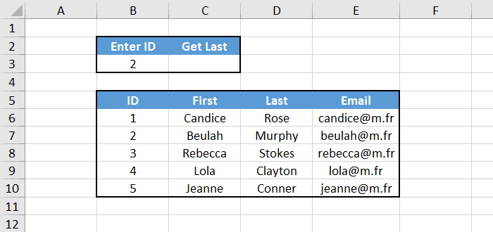
We have a small table with some information about people in it. At the top we want to extract someone's last name from his ID. We can solve that with, you guessed it, the VLOOKUP function :-)

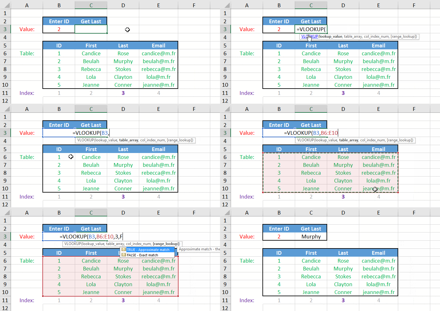
Remember all the parameters of the function? They should be like this:

• value: we are looking for someone that has an ID that match cell B3.
• table: we search in the whole people table, which is B6:E10.
• index: we want to return the last name, which is in the 3rd column of our table.
• approximate: as usuall, FALSE.

So the solution is: =VLOOKUP(B3, B6:E10, 3, FALSE)

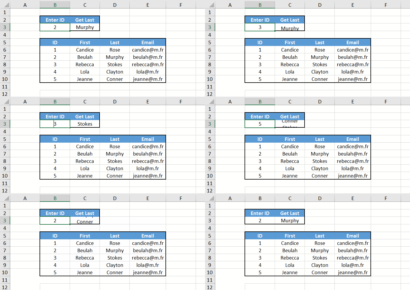
And you can see that when we change the ID in cell B3, the last name is updated correctly.

If you later change your mind and want to return the email instead of the last name, just set the index parameter to 4 and things will work fine.

Four Things to Know

And that's basically it! But before you leave, I wanted to mention 4 important things that you should know about VLOOKUP:

• The first column of the table parameter must contain the thing we are looking for, otherwise it won't work. In the example above it's the ID.
• The V at the beginning of the function name means Vertical. That's why there's also a HLOOKUP function for Horizontal searches. It works exactly the same way, except that the index parameter is for a row (instead of a column).
• In Excel, FALSE and 0 means the same thing. So for the last parameter we can use 0, which is shorter to write.
• There is a better way to extract specific data from a table in Excel, which is to combine INDEX and MATCH functions. Check out the tutorial Use Index Match to perform advanced lookups, and you will not be disappointed!

Conclusion

You know everything you need to know about the VLOOKUP function. As you see, it is quite simple use. You just need to remember what the parameters are.

• Syntax: =VLOOKUP(value, table, index, 0)
• value: the item we are searching.
• table: the table that contains the data.
• index: the column number of what we want to return.

See all the tutorials on the homepage